Unicode® Technical Standard #39
Summary
Because Unicode contains such a large number of characters and
incorporates the varied writing systems of the world, incorrect
usage can expose programs or systems to possible security attacks.
This document specifies mechanisms that can be used to detect
possible security problems.
Status
This document has been reviewed by Unicode members and other
interested parties, and has been approved for publication by the Unicode
Consortium. This is a stable document and may be used as reference
material or cited as a normative reference by other specifications.
A Unicode Technical Standard (UTS)
is an independent
specification. Conformance to the Unicode Standard does not imply
conformance to any UTS.
Please submit corrigenda and other comments with the online
reporting form [
Feedback
].
Related information that is useful in understanding this document is
found in the
References
. For the latest
version of the Unicode Standard, see [
Unicode
]. For a
list of current Unicode Technical Reports, see [
Reports
]. For more
information about versions of the Unicode Standard, see [
Versions
].
Contents
Unicode Technical Report #36, "Unicode Security
Considerations"
[
UTR36
]
provides guidelines for detecting and avoiding security problems
connected with the use of Unicode. This document specifies mechanisms
that are used in that document, and can be used elsewhere. Readers
should be familiar with [
UTR36
] before
continuing. See also the Unicode FAQ on
Security
Issues
[
FAQSec
].
An implementation claiming conformance to this specification
must do so in conformance to the following clauses:
UTS-39-C1
.
An implementation claiming to implement
the
General Profile for Identifiers
shall do so by conforming to either
UTS-39-C1-1
or
UTS-39-C1-2
.
UTS-39-C1-1
.
The Implementation shall be in accordance with the specifications in Section 3.1,
General Security Profile for Identifiers
, without change.
UTS-39-C1-2
.
The implementation shall provide a precise list of characters that are added to or removed from the profile, but otherwise be in accordance with the specifications in Section 3.1,
General Security Profile for Identifiers
.
UTS-39-C1.1
.
An implementation claiming to implement
the
IDN Security Profiles for Identifiers
shall do so by conforming to either
UTS-39-C1.1-1
or
UTS-39-C1.1-2
.
UTS-39-C1.1-1
.
The implementation shall be in accordance with the specifications in Section 3.2,
IDN Security Profiles for Identifiers
for Identifiers, without change.
UTS-39-C1.1-2
.
The implementation shall provide a precise list of characters that are added to or removed from the profile, but otherwise be in accordance with the specifications in Section 3.2,
IDN Security Profiles for Identifiers
.
UTS-39-C1.2
.
An implementation claiming to implement the
Email Security Profiles for Identifiers
shall do so by conforming to either
UTS-39-C1.2-1
or
UTS-39-C1.2-2
.
UTS-39-C1.2-1
.
The implementation shall be in accordance with the specifications in Section 3.3,
Email Security Profiles for Identifiers
, without change.
UTS-39-C1.2-2
.
The implementation shall provide a precise list of characters that are added to or removed from the profile, but otherwise be in accordance with the specifications in Section 3.3,
Email Security Profiles for Identifiers
.
UTS-39-C2
.
An implementation claiming to implement any of the following confusable-detection functions for Identifiers defined in Section 4,
Confusable Detection
shall do so by conforming to either
UTS-39-C2-1
or
UTS-39-C2-2
.
-
X and Y are single-script confusables
-
X and Y are mixed-script confusables
-
X and Y are whole-script confusables
-
X has whole-script confusables in set of scripts S
UTS-39-C2-1
.
The implementation of the function shall be in accordance with the specifications in Section 4,
Confusable Detection
, without change.
UTS-39-C2-2
.
The implementation shall provide a precise list of character mappings that are added to or removed from those provided, but otherwise be in accordance with the specifications in Section 4,
Confusable Detection
.
UTS-39-C3
.
An implementation claiming to detect mixed scripts shall do so by conforming to either
UTS-39-C3-1
or
UTS-39-C3-2
.
UTS-39-C3-1
.
The implementation shall be in accordance with the specifications in Section 5.1,
Mixed-script Detection
, without change.
UTS-39-C3-2
.
The implementation shall provide a precise description of changes in behavior, but otherwise be in accordance with the specifications in Section 5.1,
Mixed-Script Detection
.
UTS-39-C4
.
An implementation claiming to detect Restriction-Levels shall do so by conforming to either
UTS-39-C4-1
or
UTS-39-C4-2
.
UTS-39-C4-1
.
The implementation shall be in accordance with the specifications in Section 5.2,
Restriction-Level Detection
, without change.
UTS-39-C4-2
.
The implementation shall provide a precise description of changes in behavior, but otherwise be in accordance with the specifications in Section 5.2,
Restriction-Level Detection
.
UTS-39-C5
.
An implementation claiming to detect mixed numbers shall do so by conforming to either
UTS-39-C5-1
or
UTS-39-C5-2
.
UTS-39-C5-1
.
The implementation shall be in accordance with the specifications in Section 5.3,
Mixed-Number Detection
, without change.
UTS-39-C5-2
.
The implementation shall provide a precise description of changes in behavior, but otherwise be in accordance with the specifications in Section 5.3,
Mixed-Number Detection
.
Identifiers ("IDs") are strings used in application contexts
to refer to specific entities of certain significance in the given application. In a
given application, an identifier will map to at most one specific entity.
Many applications have security requirements related to identifiers.
A common example is URLs referring to pages
or other resources on the Internet: when a user wishes to access a
resource, it is important that the user can be certain what resource they
are interacting with. For example, they need to know that they are interacting with a
particular financial service and not some other entity that is spoofing the
intended service for malicious purposes. This illustrates a
general security concern for identifiers: potential ambiguity of strings.
While a machine has no difficulty distinguishing between any two different
character sequences, it could be very difficult for humans to
recognize and distinguish identifiers if an application did not limit which
Unicode characters could be in identifiers.
The focus of this specification is mitigation of such issues related
to the security of identifiers.
Deliberately restricting the characters that can be used in identifiers
is an important security technique.
The exclusion of characters from identifiers does not affect the general
use of those characters for other purposes, such as for general text in documents.
Unicode Standard Annex #31,
"Unicode Identifiers and Syntax" [
UAX31
]
provides a recommended method of determining which strings should
qualify as identifiers. The UAX #31 specification extends the common
practice of defining identifiers in terms of letters and numbers to
the Unicode repertoire.
That specification also permits other protocols to use that method as
a base, and to define a
profile
that adds or removes
characters. For example, identifiers for specific programming
languages typically add some characters like "$", and
remove others like "-" (because of the use as
minus
),
while IDNA removes "_" (among others)—see Unicode
Technical Standard #46, "Unicode IDNA Compatibility
Processing" [
UTS46
], as well as [
IDNA2003
], and [
IDNA2008
].
This document provides for additional identifier profiles for
environments where security is an issue. These are profiles of the
extended identifiers based on properties and specifications of the
Unicode Standard [
Unicode
], including:
-
The XID_Start and XID_Continue properties defined in the
Unicode Character Database (see [
DCore
])
-
The toCasefold(X) operation defined in
Chapter
3, Conformance
of [
Unicode
]
-
The NFKC and NFKD normalizations defined in
Chapter
3, Conformance
of [
Unicode
]
The data files used in defining these profiles follow the UCD File
Format, which has a semicolon-delimited list of data fields
associated with given characters, with each field referenced by
number. For more details, see [
UCDFormat
].
The files under [
idmod
] provide data for a profile of
identifiers in environments where security is at issue. The files
contain a set of characters recommended to be restricted from use.
They also contain a small set of characters that are recommended as
additions to the list of characters defined by the XID_Start and
XID_Continue properties, because they may be used in identifiers in a
broader context than programming identifiers.
The Restricted characters are characters not in common use, and
they can be blocked to further reduce the possibilities for visual
confusion. They include the following:
-
characters not in modern use
-
characters only used in specialized fields, such as
liturgical characters, phonetic letters, and mathematical
letter-like symbols
-
characters in limited use by very small communities
The choice of which characters to specify as Restricted starts conservatively, but allows additions
in the future as requirements for characters are refined.
For information on handling modifications
over time, see
Section 2.10.1, Backward
Compatibility
in
Unicode Technical Report #36,
"Unicode Security Considerations"
[
UTR36
].
An implementation following the General Security Profile does not
permit any characters in \p{Identifier_Status=Restricted}, unless it documents the
additional characters that it does allow. Such documentation can specify characters via properties, such as \p{Identifier_Type=Technical}, or by explicit lists, or by combinations of these. Implementations may also specify that fewer characters are allowed than implied by \p{Identifier_Status=Allowed}; for example, they can allow only characters permitted by [
IDNA2008
].
Common candidates for such
additions include characters for scripts listed in
Table 7,
Limited Use Scripts
of [
UAX31
]. However,
characters from these scripts have not been a priority for
examination for confusables or to determine specialized, non-modern,
or uncommon-use characters.
Canonical equivalence is applied when testing candidate identifiers
for inclusion of
Allowed
characters. For example, suppose
the candidate string is the sequence
<u,
combining-diaeresis
>
The target string would be Allowed in
either
of the
following 2 situations:
-
u is Allowed and ¨ is Allowed, or
-
ü is Allowed
For details of the format for the [
idmod
] files, see
Section 7,
Data Files
.
Table 1.
Identifier_Status and Identifier_Type
|
Identifier_Status
|
Identifier_Type
|
Description
|
|
Restricted
|
Not_Character
|
Unassigned characters, private use characters,
surrogates, non-whitespace control characters.
|
|
Deprecated
|
Characters with the Unicode property
Deprecated=Yes
.
|
|
Default_Ignorable
|
Characters with the Unicode property
Default_Ignorable_Code_Point=Yes
.
|
|
Not_NFKC
|
Characters that cannot occur in strings
normalized to NFKC.
|
|
Not_XID
|
Characters that do not qualify as
default Unicode identifiers; that is, they do not have the Unicode
property
XID_Continue=True
.
|
|
Exclusion
|
Characters with Script_Extensions values containing a script in
Table 4,
Excluded Scripts
from [
UAX31
], and no script from
Table 7,
Limited Use Scripts
or
Table 5,
Recommended Scripts
, other than “Common” or “Inherited”.
|
|
Obsolete
|
Characters that are no longer in modern use,
or that are not commonly used in modern text.
|
|
Technical
|
Specialized usage: technical, liturgical, etc.
|
|
Uncommon_Use
|
Characters that are uncommon, or are limited in use (even though they are in scripts that are not "Limited_Use"), or whose usage is uncertain.
May be combined with Exclusion or Limited_Use for
characters that are less common than the main characters of their scripts.
|
|
Limited_Use
|
Characters from scripts that are in limited
use: with Script_Extensions values containing a script in
Table 7,
Limited Use Scripts
in [
UAX31
], and no script from
Table 5,
Recommended Scripts
,
other than “Common” or “Inherited”.
|
|
Allowed
|
Inclusion
|
Exceptionally allowed characters, including
Table 3a,
Optional Characters for Medial
and
Table 3b,
Optional Characters for Continue
in [
UAX31
], and some characters for [
IDNA2008
], except for certain characters that are Restricted above.
|
|
Recommended
|
Characters from scripts that are in widespread everyday common use:
with Script_Extensions values containing a script in
Table 5,
Recommended Scripts
in [
UAX31
], except for those characters that are Restricted above.
|
Note:
In Unicode 15.0, the Join_Control characters (ZWJ/ZWNJ) have been removed from
Identifier_Type=
Inclusion
.
They thereby have the properties
Identifier_Type=
Default_Ignorable
and
Identifier_Status=
Restricted
.
Their inclusion in programming language identifier profiles has usability and security implications.
Implementations of the General Profile for Identifiers that wish to retain ZWJ and ZWNJ should declare that they use a modification of the profile per
Section 2, Conformance
,
and should ensure that they implement the restrictions described in
Section 3.1.1, Joining Controls
.
Identifier_Status and Identifier_Type are properties of characters (code points).
See
UTS #18: Unicode Regular Expressions
[
UTS18
]
and
UTR #23: The Unicode Character Property Model
[
UTR23
] for
more discussion.
For the purpose of regular expressions,
the long and short names of these properties and their values
are documented in their respective data files;
see
Section 7,
Data Files
.
For stability considerations, see
Migrating
Persistent Data
.
There may be multiple reasons for restricting a character; therefore,
the Identifier_Type property allows multiple values that correspond with
Restricted. For example, some characters have Identifier_Type values of
Limited_Use and Technical. Multiple values are not assigned to characters with strong restrictions: Not_Character, Deprecated, Default_Ignorable, Not_NFKC. For
example, if a character is Deprecated, there is little value in also
marking it as Uncommon_Use. For the qualifiers on usage, Obsolete,
Uncommon_Use and Technical, the distinctions among the Identifier_Type values is not strict and
only one might be given. The important characteristic is the Identifier_Status:
whether or not the character is Restricted.
The default Identifier_Type property value should be Uncommon_Use if no other categories apply.
See
Section 3.1.2,
Choosing Identifier_Type Values
.
As more
information is gathered about characters, this data may change in
successive versions.
That can cause either the Identifier_Status
or Identifier_Type to change for a particular character. Thus users of
this data should be prepared for changes in successive versions, such
as by having a backward compatibility policy in place for previously
supported characters or registrations. Both Identifier_Status
and Identifier_Type values are to be compared
case-insensitively and ignoring hyphens and underbars.
Restricted characters should be treated with caution when considering possible use in identifiers,
and should be disallowed unless there is good reason to allow them in the
environment in question. However, the set of Identifier_Status=Allowed
characters are not typically used as is by implementations. Instead,
they are applied as filters to the set of characters C that are
supported by the identifier syntax, generating a new set C′.
Typically there are also particular characters or classes of
characters from C that are retained as
Exception
characters.
C′ = (C ∩ {Identifier_Status=Allowed}) ∪
Exception
The implementation may simply restrict use of new identifiers to C′,
or may apply some other strategy. For example, there might be an
appeal process for registrations of ids that contain characters
outside of C′ (but still inside of C), or in user interfaces for
lookup of identifiers, warnings of some kind may be appropriate. For
more information, see [
UTR36
].
The
Exception
characters would be
implementation-specific. For example, a particular implementation
might extend the default Unicode identifier syntax by adding
Exception
characters with the Unicode property
XID_Continue=False
,
such as “$”, “-”, and “.”. Those characters are specific to that
identifier syntax, and would be retained even though they are not in
the Identifier_Status=Allowed set. Some
implementations may also wish to add some [
CLDR
]
exemplar characters for particular supported languages that have
unusual characters.
The Identifier_Type=Inclusion characters already
contain some characters that are not letters or numbers, but that are
used within words in some languages. For example, it is recommended
that U+00B7 (·) MIDDLE DOT be allowed in identifiers, because it is
required for Catalan.
The implementation may also apply other restrictions discussed
in this document, such as checking for confusable characters or doing
mixed-script detection.
Visible distinctions
created by certain characters excluded by the
General Security Profile because their Identifier_Type is Default_Ignorable (particularly the
Join_Control
characters
) are necessary in certain languages. A blanket exclusion
of these characters makes it impossible to create identifiers with
the correct visual appearance for common words or phrases in those
languages.
Identifier systems that attempt to provide more natural
representations of terms in "modern, customary usage"
should allow these characters in input and display, but limit them to
contexts in which they are necessary. The term
modern
customary usage
includes characters that are in common use in
newspapers, journals, lay publications; on street signs; in
commercial signage; and as part of common geographic names and
company names, and so on. It does not include technical or academic
usage such as in mathematical expressions, using archaic scripts or
words, or pedagogical use (such as illustration of half-forms or
joining forms in isolation), or liturgical use.
The goals for such a restriction of format characters to
particular contexts are to:
-
Allow the use of these characters where required in normal
text
-
Exclude as many cases as possible where no visible
distinction results
-
Be simple enough to be easily implemented with standard
mechanisms such as regular expressions
An implementation following the General Security Profile that allows the additional characters ZWJ and ZWNJ shall only permit them where they
satisfy the conditions A1, A2, and B in
Section 3.1.1.1,
Limited Contexts for Joiner Controls
, unless it documents the
additional contexts where it allows them.
More advanced implementations may use script-specific information for more detailed testing. In particular, they can:
1.
Disallow joining controls
in sequences that meet the conditions of A1, A2, and B, where in common fonts the resulting appearance of the sequence is normally not distinct from appearance in the same sequences with the joining controls removed.
2.
Allow joining controls
in sequences that don't meet the conditions of A1, A2, and B, where in common fonts the resulting appearance of the sequence is normally distinct from the appearance in the same sequences with the joining controls removed. The following regular expressions describe sequences that typically result in distinct rendering. They use the notation explained below in
A1
.
/$L ZWNJ $V $L/
/$L ZWJ $V $L/
An implementation that
attempts to provide more natural representations of terms in "modern, customary usage" should allow the
following Join_Control characters in the limited contexts specified
in
A1
,
A2
, and
B
below.
U+200C ZERO WIDTH NON-JOINER (ZWNJ)
U+200D ZERO WIDTH JOINER
(ZWJ)
There are also two global conditions incorporated in each of
A1
,
A2
, and
B
:
-
Script Restriction.
In each of the following cases,
the specified sequence must only consist of characters from a single
script (after ignoring
Common
and
Inherited
script
characters).
-
Normalization.
In each of the following cases, the
specified sequence must be in NFC format. (To test an identifier
that is not required to be in NFC, first transform into NFC format
and then test the condition.)
Implementations may also impose tighter restrictions than provided below, in order to eliminate some other circumstances where the characters either have no visual effect or the effect has no semantic importance.
A1
. Allow ZWNJ in the
following context:
Breaking a cursive connection.
That is, in the context based
on the Joining_Type property, consisting of:
-
A Left-Joining or Dual-Joining character, followed by zero
or more Transparent characters, followed by a ZWNJ,
followed by a Right-Joining or
Dual-Joining character
This corresponds to the following regular expression (in Perl-style
syntax):
/$LJ $T* ZWNJ $RJ/
Where the character classes like $T could be
defined with Unicode properties
(similar to UnicodeSet notation) like this:
$T = \p{Joining_Type=Transparent}
$RJ =
[\p{Joining_Type=Dual_Joining}\p{Joining_Type=Right_Joining}]
$LJ = [\p{Joining_Type=Dual_Joining}\p{Joining_Type=Left_Joining}]
For example, consider the Persian word <
Noon, Alef, Meem, Heh, Alef, Farsi Yeh
>. Without a ZWNJ, it translates to "names of",
as shown in the first row; with a ZWNJ between
Heh
and
Alef
, it means
"a letter", as shown in the second row of
Figure 1
.
Figure 1.
Persian Example with
ZWNJ
A2
. Allow ZWNJ in the
following context:
In a conjunct context.
That is, a sequence of the form:
-
A Letter, followed by a Virama, followed by a ZWNJ (optionally preceded or followed by certain nonspacing marks), followed by a Letter.
This corresponds to the following regular expression (in Perl-style
syntax):
/$L $M* $V $M₁* ZWNJ $M₁* $L/
Where:
$L = \p{General_Category=Letter}
$V =
\p{Canonical_Combining_Class=Virama}
$M = \p{General_Category=Mn}
$M₁ = [\p{General_Category=Mn}&\p{CCC≠0}]
For example, the Malayalam word for
eyewitness
is shown in
Figure
2
. The form without the ZWNJ in the second row is incorrect in this
case.
Figure 2.
Malayalam Example
with ZWNJ
B
. Allow ZWJ in the
following context:
In a conjunct context.
That is, a sequence of the form:
-
A Letter, followed by a Virama, followed by a ZWJ (optionally preceded or followed by certain nonspacing marks), and not followed by a character of type Indic_Syllabic_Category=Vowel_Dependent
This corresponds to the following regular expression (in Perl-style
syntax):
/$L $M* $V $M₁* ZWJ (?!$D)/
Where:
$L= \p{General_Category=Letter}
$V =
\p{Canonical_Combining_Class=Virama}
$M = \p{General_Category=Mn}
$M₁ = [\p{General_Category=Mn}&\p{CCC≠0}]
$D = \p{Indic_Syllabic_Category=Vowel_Dependent}
For example, the Sinhala word for the country 'Sri Lanka' is
shown in the first row of
Figure 3
, which uses both a space
character and a ZWJ. Removing the space results in the text shown in
the second row of
Figure 3
, which is still legible, but
removing the ZWJ completely modifies the appearance of the
'Sri' cluster and results in the unacceptable text appearance
shown in the third row of
Figure 3
.
Figure 3.
Sinhala Example with
ZWJ
Note:
The restrictions in
A1
,
A2
, and
B
are more restrictive than the CONTEXTJ rules defined in
Appendix A, Contextual Rules Registry
,
in
The Unicode Code Points and Internationalized Domain Names for Applications (IDNA)
[
IDNA2008
]. In particular,
A1
does not allow
transparent characters after the ZWNJ, while
A2
and
B
require an extended context
indicating an actual conjunct cluster rather than merely
a single preceding virama. Consequently,
any identifier that satisfies these constraints also
satisfies the CONTEXTJ rules for joining controls in
IDNs. Note that many registries impose additional restrictions
on permissible IDNs beyond those required by
CONTEXTJ.
While the restrictions in
A1
,
A2
, and
B
greatly
limit visual confusability, they do not prevent it. For example,
because Tamil only uses a Join_Control character in one specific
case, most of the sequences these rules allow in Tamil are, in fact,
visually confusable. Therefore based on their knowledge of the script
concerned, implementations may choose to have tighter restrictions
than specified in
Section 3.1.1.1,
Limited Contexts for Joining Controls
—for example, by explicitly providing for the exceptional sequence, while otherwise disallowing the joiner in context.
There are also cases where a joiner preceding a
virama makes a visual distinction in some scripts. It is currently
unclear whether this distinction is important enough in identifiers
to warrant retention of a joiner. For more information, see UTR #36:
Unicode Security Considerations
[
UTR36
].
Performance.
Parsing identifiers can be a
performance-sensitive task. However, these characters are quite rare
in practice, thus the regular expressions (or equivalent processing)
only rarely would need to be invoked. Thus these tests should not add
any significant performance cost overall.
The following identifier types may be assigned singly or in combination.
The values are based on best available information and may be updated when new information becomes available.
Multiple classifications may be possible,
particularly where a character is of one type in a commonly used writing system
and of different type in another context.
-
Uncommon_Use
focuses on usage of the character in orthographies for living languages.
Uncommon_Use can also represent the absence of confirmed or credible data
on a level of usage that would correspond to “common everyday use” for an orthography in widespread use.
Uncommon_Use is the default for newly encoded characters for all scripts other than Excluded scripts,
unless a sufficient level of usage can be confirmed for one or more specific orthographies
in common modern use.
-
Where combining marks, such as
U+3099 COMBINING KATAKANA-HIRAGANA VOICED SOUND MARK,
are only needed for the NFD form of recommended characters,
they have been given the Identifier_Type Uncommon_Use.
Identifier systems that work with unnormalized text, or text in NFD,
may wish to add the full set of characters required in canonical decompositions.
-
Obsolete
focuses on the degree to which a character is in common modern use.
If a writing system, or an orthography using a character, has fallen out of use,
or a character is no longer used in a given context, it is marked Obsolete.
A character can become obsolete in the context of a writing system;
it is not required that the entire writing system has fallen out of use.
A character may be Obsolete in a widely used writing system,
but also part of an orthography where it is in Uncommon_Use.
-
Technical
focuses on the purpose of use.
If a character is limited to particular types of texts or
forms part of a notation that is not in everyday use,
then it would be appropriate to categorize it as Technical.
Technical uses can include liturgical texts, poetry, phonetic notation, and so on.
A character may have a common technical use, but
may also be used in one or more orthographies at a level that is marked by Uncommon_Use,
or it could be Obsolete as a character for general use.
-
Inclusion
focuses on
Allowed
punctuation
and characters that look like punctuation.
For each identifier environment they should be carefully reviewed,
as some or all of them may not be suitable for that environment:
For example, when a character is, or can be confused with,
a syntax character in the given environment.
The other identifier types are largely, if not fully,
determined by a character’s other property values and are therefore automatically assigned.
Version 1 of this document defined operations and data that apply to
[
IDNA2003
], which has been superseded by [
IDNA2008
] and Unicode Technical
Standard #46, "Unicode IDNA Compatibility
Processing" [
UTS46
]. The identifier
modification data can be applied to whichever specification of IDNA
is being used. For more information, see the [
IDN
FAQ
].
However, implementations can claim conformance to other features of
this document as applied to domain names, such as
Restriction Levels
.
In addition, there are other specifications that are extremely useful for IDNs.
Notably, RFC7940 specifies a machine-readable format
for expressing profiles for IDNs with specific features that support security against spoofing.
Such profiles are known as “Label Generation Rules” (LGR) and are typically defined for a script or language,
with features that allow support of multiple LGRs for the same “DNS zone”.
Using the LGR format, implementations can:
-
Select a repertoire of characters or enumerated character sequences.
The selection of the set of characters can take into account
the intersection between IDNA2008 allowed values and
Identifier_Status resp. Identifier_Type.
-
Limit certain characters to one or more of an enumerated set of sequences.
That’s useful to limit diacritics to contexts where they are expected,
or to exclude standalone use of some characters only found in certain sequences.
-
Provide a context rule.
A context rule is an anchored regular expression
describing either a required or prohibited context for
a character or sequence inside a label.
This is useful for restrictions on Indic scripts,
so you can stay within safe boundaries of what rendering engines can render in a distinct way.
One application is to implement
Limited Contexts for Joining Controls
.
-
Make two characters / sequences “blocked” variants of each other.
Either one is allowed, but the first label registered blocks
the label differing only by a variant character or sequence at that position.
-
Use a “whole label evaluation” rule to validate an identifier.
A WLE rule is a regular expression describing a pattern either for a valid or an invalid label.
This can be used, for example, to prevent digit set mixing in the same label,
or making sure a label is consistent in the choice of a regional alternative for a character.
The LGR mechanism, as defined in RFC 7940,
allows you to present all of these restrictions in a
machine-readable form which you can then convert into
whatever works best for validating and resolving
competing identifier registrations in your system (or symbol table).
The format was designed with IDNA2008 in mind and is used in
the normative definition of IDN profiles for the DNS Root Zone.
In RFC7940, the regular expressions can be specified in terms of
Unicode properties or custom attributes assigned to the characters in the LGR.
The same mechanisms can be applied to other types of identifiers.
More information can be found at [
ICANN
].
The
SMTP Extension for Internationalized Email
provides for specifications of internationalized email addresses [
EAI
]. However, it does not provide for testing those addresses for security issues. This section provides an email security profile that may be used for that. It can be applied for different purposes, such as:
-
When an email address is registered, flag anything that
does not meet the profile:
-
Either forbid the registration, or
-
Allow for an appeals process.
-
When an email address is detected in linkification of plain
text:
-
Do not linkify if the identifier does not meet
the profile.
-
When an email address is displayed in incoming email:
-
Flag it as suspicious with a wavy underline, if it
does not meet the profile.
-
Filter characters from the quoted-string-part to prevent
display problems.
This profile does not exclude characters from
EAI. Instead, it provides a profile that can be used for registration, linkification,
and notification. The goal is to flag
addresses that are structurally unsound or contain unexpected detritus.
An email address is formed from three main parts. (There are more elements of an email address, but these are the ones for which Unicode security is important.) For example:
"Joey" <joe31834@gmail.com>
-
The
domain-part
is "gmail.com"
-
The
local-part
is "joe31834"
-
The
quoted-string-part
is "Joey"
To meet the requirements of the
Email Security Profiles for Identifiers
section of this specification, an identifier must satisfy the following
conditions for the specified <restriction level>.
Domain-Part
The domain-part of an email address must satisfy
Section 3.2,
IDN
Security Profiles for Identifiers
, and satisfy the conformance
clauses of [
UTS46
].
Local-Part
The local-part of an email address must satisfy all the following conditions:
-
It must be in NFKC format
-
It must have level = <restriction level> or less,
from
Restriction_Level_Detection
-
It must not have mixed number systems according to
Mixed_Number_Detection
-
It must satisfy
dot-atom-text
from
RFC
5322 §3.2.3
, where
atext
is extended as follows:
Where C ≤ U+007F, C is defined as in
§3.2.3
.
(That is, C ∈ [
!#-'*+\-/-9=?A-Z\^-~
].
This list copies what is already in §3.2.3,
and follows
HTML5
for ASCII.)
Where C > U+007F, both of the following conditions
are true:
-
C has Identifier_Status=Allowed from
General Security Profile
-
If C is the first character, it must be XID_Start from
Default Identifier_Syntax
in [
UAX31
]
Note that in
RFC
5322 §3.2.3
:
    dot-atom-text   =
              1*atext *("." 1*atext)
That is, dots can also occur in the local-part, but
not leading, trailing, or two in a row. In more conventional regex syntax, this would be:
    dot-atom-text   =
        atext+ ("." atext+)*
Note that bidirectional controls and other format characters are
specifically disallowed in the local-part, according to the
above.
Quoted-String-Part
The quoted-string-part of an email address must
satisfy the following conditions:
-
It must be in NFC.
-
It must not contain any stateful bidirectional format characters.
-
That is, no [:bidicontrol:] except for the LRM, RLM, and ALM, since the bidirectional controls could influence the ordering of characters outside
the quotes.
-
It must not contain more than four nonspacing marks in a row, and no
sequence of two of the same nonspacing marks.
-
It may contain mixed scripts, symbols (including emoji),
and so on.
Other Issues
The restrictions above are insufficient to
prevent bidirectional-reordering that could intermix the quoted-string-part
with the local-part or the domain-part in display. To prevent that,
implementations could use bidirectional isolates (or equivalent) around
each of these parts in display.
Implementations may also want to use other checks, such as for confusability, or services such as Safe Browsing.
A serious practical issue is that clients do not know what the
identity rules are for any particular email server: that is, when two
email addresses are considered equivalent. For example, are
mark@macchiato.com
and
Mark@macchiato.com
treated the same by the server?
Unfortunately, there is no way to query a server to see
what identity rules it follows. One of the techniques used to deal with
this problem is having whitelists of email providers indicating which of them are case-insensitive, dot-insensitive, or both.
The data in [
confusables
] provide a
mechanism for determining when two strings are visually confusable.
The data in these files may be refined and extended over time. For
information on handling modifications over time, see
the
Migration
section of this document.
The data provides a mapping from source characters to their prototypes. A prototype should be thought of as a sequence of one or more classes of symbols, where each class has an exemplar character. For example, the character U+0153 (œ), LATIN SMALL LIGATURE OE, has a prototype consisting of two symbol classes: the one with exemplar character U+006F (o), and the one with exemplar character U+0065 (e). If an input character does not have a prototype explicitly defined in the data file, the prototype is assumed to consist of the class of symbols with the input character as the exemplar character.
For an input string X, define
internalSkeleton
(X) to be the following transformation on the string:
-
Convert X to NFD format, as described in [
UAX15
].
-
Remove any characters in X that have the property Default_Ignorable_Code_Point.
-
Concatenate the prototypes for each character in X according to the specified data, producing a string of exemplar characters.
-
Reapply NFD.
For an input string X and a direction 𝑑 ∈ {RTL, LTR, FS}, define bidiSkeleton(𝑑, X) to be the following transformation on the string:
-
Reorder the code points in X for display by applying the rules of the Unicode Bidirectional Algorithm [
UAX9
] up to and including L2, treating X in isolation; if 𝑑≠FS, apply protocol HL1 to set the paragraph level to 1 if 𝑑=RTL, and to 0 if 𝑑=LTR; this yields the reordered sequence of characters R.
-
Apply rule L3 of the UBA: move combining marks after their base in R; this yields the sequence R′.
-
Replace any character whose glyph would be mirrored by rule L4 of the UBA by the value of its Bidi_Mirroring_Glyph property, yielding R″.
-
bidiSkeleton(𝑑, X) is then internalSkeleton(R″).
The strings X and Y are defined to be 𝑑-confusable if and only if bidiSkeleton(𝑑, X) = bidiSkeleton(𝑑, Y). This is abbreviated as X ≒ Y (𝑑).
This mechanism imposes transitivity on the data, so if X ≒ Y (𝑑) and Y ≒ Z (𝑑), then X ≒ Z (𝑑). It is possible to provide a more sophisticated confusable detection, by providing a metric between given characters, indicating their "closeness." However, that is computationally much more expensive, and requires more sophisticated data, so at this point in time the simpler mechanism has been chosen. That means that in some cases the test may be overly inclusive.
Note:
The operation
internalSkeleton
may change the Bidi_Class of characters, so it does not commute with the reordering and mirroring steps, and needs to be performed after them.
Example:
The sequences of code points S₁ and S₂ are LTR-confusable:
S₁ ≔ "A1<שׂ" = (LATIN CAPITAL LETTER A, DIGIT ONE, LESS-THAN SIGN, HEBREW LETTER SHIN, HEBREW POINT SIN DOT)
S₂ ≔ "Αשֺ>1" = (GREEK CAPITAL LETTER ALPHA, HEBREW LETTER SHIN, HEBREW POINT HOLAM HASER FOR VAV, GREATER-THAN SIGN, DIGIT ONE)
Computation of bidiSkeleton(LTR, S₁):
R₁ = (LATIN CAPITAL LETTER A, DIGIT ONE, LESS-THAN SIGN, HEBREW POINT SIN DOT, HEBREW LETTER SHIN)
R′₁ = (LATIN CAPITAL LETTER A, DIGIT ONE, LESS-THAN SIGN, HEBREW LETTER SHIN, HEBREW POINT SIN DOT)
R″₁ = (LATIN CAPITAL LETTER A, DIGIT ONE, LESS-THAN SIGN, HEBREW LETTER SHIN, HEBREW POINT SIN DOT)
bidiSkeleton(LTR, S₁) = internalSkeleton(R″₁) = (LATIN CAPITAL LETTER A, LATIN SMALL LETTER L, LESS-THAN SIGN, HEBREW LETTER SHIN, COMBINING DOT ABOVE)
Computation of bidiSkeleton(LTR, S₂):
R₂ = (GREEK CAPITAL LETTER ALPHA, DIGIT ONE, GREATER-THAN SIGN, HEBREW POINT HOLAM HASER FOR VAV, HEBREW LETTER SHIN)
R′₂ = (GREEK CAPITAL LETTER ALPHA, DIGIT ONE, GREATER-THAN SIGN, HEBREW LETTER SHIN, HEBREW POINT HOLAM HASER FOR VAV)
R″₂ = (GREEK CAPITAL LETTER ALPHA, DIGIT ONE, LESS-THAN SIGN, HEBREW LETTER SHIN, HEBREW POINT HOLAM HASER FOR VAV)
bidiSkeleton(LTR, S₂) = internalSkeleton(R″₂) = (LATIN CAPITAL LETTER A, LATIN SMALL LETTER L, LESS-THAN SIGN, HEBREW LETTER SHIN, COMBINING DOT ABOVE)
Note that these sequences are not RTL-confusable; indeed in a right-to-left paragraph, the strings look distinct:
S₁ = "
A1<שׂ
"
S₂ = "
Αשֺ>1
"
LTR, and RTL, and FS confusability should be used when it is inappropriate to enforce that strings be single-script,
or at least single-directionality; this is the case in programming language identifiers.
See
Section 5.1, Confusability Mitigation Diagnostics
, in
Unicode Technical Standard #55, Unicode Source Code Handling
[
UTS55
].
The bidiSkeleton is costlier to compute than the internalSkeleton, as the bidirectional algorithm must be applied.
However, a fast path can be used: if 𝑑=LTR and X has no characters with bidi classes R or AL, bidiSkeleton(𝑑, X) = internalSkeleton(X).
Further, if the strings are known not to contain explicit directional formatting characters (as is the case for UAX31-R1 Default Identifiers
defined in
Unicode Standard Annex #31, Unicode Identifiers and Syntax
[
UAX31
]), the algorithm can be drastically simplified,
as the X rules are trivial, obviating the need for the directional status stack of the Unicode Bidirectional Algorithm.
The highest possible resolved level is then 2; see
Table 5, Resolving Implicit Levels
,
in
Unicode Standard Annex #9, Unicode Bidirectional Algorithm
[
UAX9
].
Note:
The strings
bidiSkeleton
(𝑑, X) and
bidiSkeleton
(𝑑, Y)
are
not
intended for display.
Further, they are not stable across versions of Unicode, so that
they can only be interchanged between systems that use the same version of Unicode to compute
bidiSkeleton
.
If they are stored, they must be recomputed when updating the version of Unicode used to compute
bidiSkeleton
.
They should be thought of as an intermediate processing form,
similar to a hashcode. The exemplar characters are
not
guaranteed to be identifier characters.
The use of bidirectional confusability with an appropriate direction is preferable when possible.
However, for cases where the direction with which identifiers will be displayed is unknown,
and for compatibility with earlier definitions of confusability which did not take bidirectional reordering into account,
the operation
skeleton
is
defined as skeleton(X) = bidiSkeleton(LTR, X). The strings X and Y are then
defined to be
confusable
if and only if skeleton(X) = skeleton(Y). This is abbreviated as X ≅ Y.
Note:
Some implementations of confusable detection outside Unicode use different terminology.
In particular, in the ICANN Root Zone Label Generation Rules [
RZLGR5
], the term
variant of X
is used for a property similar to
confusable with X
, and the term
index variant
is used for the equivalent of
skeleton
.
Definitions
Confusables are divided into three classes: single-script confusables, mixed-script confusables, and whole-script confusables, defined below. All confusables are either a single-script confusable or a mixed-script confusable, but not both. All whole-script confusables are also mixed-script confusables.
The definitions of these three classes of confusables depend on the definitions of
resolved script set
and
single-script
, which are provided in
Section 5,
Mixed-Script
Detection
.
X and Y are
single-script confusables
if
and only if they are confusable, and their resolved script sets have at least one element in common.
Examples: “ljeto” and “ljeto” in Latin (the Croatian word for “summer”), where the first word uses only four codepoints, the first of which is U+01C9 (lj) LATIN SMALL LETTER LJ.
X and Y are
mixed-script confusables
if
and only if they are confusable but their resolved script sets have no elements in common.
Examples: "paypal" and "pаypаl", where the
second word has the character
U+0430
( а )
CYRILLIC SMALL LETTER A.
X and Y are
whole-script confusables
if
and only if they are
mixed-script confusables,
and each of them is a
single-script string.
Example: "scope" in Latin and "ѕсоре" in Cyrillic.
As noted in Section 5, the resolved script set ignores characters with Script_Extensions {Common} and {Inherited} and augments characters with CJK scripts with their respective writing systems. Characters with the
Script_Extensions property values COMMON or
INHERITED are ignored when testing for differences in script.
Data File Format
Each line in the data file has the following format: Field 1 is
the source, Field 2 is the target, and Field 3 is obsolete, always containing the letters “MA” for backwards compatibility. For example:
0441 ; 0063 ; MA # ( с → c ) CYRILLIC SMALL LETTER ES → LATIN SMALL
LETTER C #
2CA5 ; 0063 ; MA # ( ⲥ → c ) COPTIC SMALL LETTER SIMA → LATIN
SMALL LETTER C # →ϲ→
Everything after the # is a comment and is purely informative. An
asterisk after the comment indicates that the character is not an XID
character [
UAX31
]. The comments provide the
character names.
Implementations that use the confusable data do not have to
recursively apply the mappings, because the transforms are
idempotent. That is,
internalSkeleton(internalSkeleton(X)) = internalSkeleton(X)
If the data was derived via transitivity, there is
an extra comment at the end. For instance, in the above example the
derivation was:
-
ⲥ (U+2CA5 COPTIC SMALL LETTER SIMA)
-
→ ϲ (U+03F2 GREEK LUNATE SIGMA SYMBOL)
-
→ c (U+0063 LATIN SMALL LETTER C)
The data may change between versions. Even where the data is the
same, the order of lines in the files may change between versions.
For more information, see
Migration
.
Note:
Due to production problems, versions
before 7.0 did not maintain idempotency in all cases. For more
information, see
Migration
.
For some applications, it is useful to determine if a given input string has any whole-script confusable. For example, the identifier "ѕсоре" using Cyrillic characters would pass the single-script test described in
Section 5.2,
Restriction-Level Detection
, even though it is likely to be a spoof attempt.
It is possible to determine whether a single-script string X has a whole-script confusable:
-
Consider Q, the set of all strings that are confusable with X.
-
Remove all strings from Q whose resolved script set intersects with the resolved script set of X.
-
If Q is nonempty and contains any single-script string, return TRUE.
-
Otherwise, return FALSE.
The logical description above can be used for a reference implementation for testing, but is not particularly efficient. A production implementation can be optimized as long as it produces the same results.
Note that the confusables data include a large number of mappings between Latin and Cyrillic text. For this reason, the above algorithm is likely to flag a large number of legitimate strings written in Latin or Cyrillic as potential whole-script confusables. To effectively use whole-script confusables, it is often useful to determine both whether a string has a whole-script confusable, and
which
scripts those whole-script confusables have.
This information can be used, for example, to distinguish between reasonable versus suspect whole-script confusables. Consider the Latin-script domain-name label “circle”. It would be appropriate to have that in the domain name “circle.com”. It would also be appropriate to have the Cyrillic confusable “сігсӀе” in the Cyrillic domain name “сігсӀе.рф”. However, a browser may want to alert the user to possible spoofs if the Cyrillic “сігсӀе” is used with .com or the Latin “circle” is used with .рф.
The process of determining suspect usage of whole-script confusables is more complicated than simply looking at the scripts of the labels in a domain name. For example, it can be perfectly legitimate to have scripts in a SLD (second-level domain) not be the same as scripts in a TLD (top-level domain), such as:
-
Cyrillic labels in a domain name with a TLD of .ru or .рф
-
Chinese labels in a domain name with a TLD of .com.au or .com
-
Cyrillic labels
that aren’t confusable
with Latin with a TLD of .com.au or .com
The following high-level algorithm can be used to determine all scripts that contain a whole-script confusable with a string X:
-
Consider Q, the set of all strings confusable with X.
-
Remove all strings from Q whose resolved script set is ∅ or
ALL
(that is, keep only single-script strings plus those with characters only in Common).
-
Take the union of the resolved script sets of all strings remaining in Q.
As usual, this algorithm is intended only as a definition; implementations should use an optimized routine that produces the same result.
To determine the existence of a mixed-script confusable, a similar process could be used:
-
Consider Q, the set of all strings that are confusable with X.
-
Remove all strings from Q whose resolved script set intersects with the resolved script set of X.
-
If Q is nonempty, return TRUE.
-
Otherwise, return FALSE.
The logical description above can be used for a reference implementation for testing, but is not particularly efficient. A production implementation can be optimized as long as it produces the same results.
Note that due to the number of mappings provided by the confusables data, the above algorithm is likely to flag a large number of legitimate strings as potential mixed-script confusables.
The Unicode Standard supplies information that can be used for
determining the script of characters and detecting mixed-script text.
The determination of script is according to the
UAX #24, Unicode Script Property
[
UAX24
], using data from the Unicode Character Database [
UCD
].
Define a character's
augmented script set
to be a character's Script_Extensions with the following two modifications.
-
Entries for the writing systems containing multiple scripts — Hanb (Han with Bopomofo),
Hntl (Traditional Han with Latin), Jpan (Japanese), and Kore (Korean) — are added according to the following rules.
-
If Script_Extensions contains Hani (Han), add Hanb,
Hntl, Jpan, and Kore.
-
If Script_Extensions contains Hira (Hiragana), add Jpan.
-
If Script_Extensions contains Kana (Katakana), add Jpan.
-
If Script_Extensions contains Hang (Hangul), add Kore.
-
If Script_Extensions contains Bopo (Bopomofo), add Hanb.
-
If Script_Extensions contains Latn
(Latin), add Hntl.
-
Sets containing Zyyy (Common) or Zinh (Inherited) are treated as
ALL
, the set of all script values.
The Script_Extensions data is from the Unicode Character Database [
UCD
]. For more information on the Script_Extensions property and Jpan, Kore,
Hntl, and Hanb, see
UAX #24, Unicode Script Property
[
UAX24
].
Define the
resolved script set
for a string to be the intersection of the augmented script sets over all characters in the string.
A string is defined to be
mixed-script
if its resolved script set is empty and defined to be
single-script
if its resolved script set is nonempty.
Note:
The term “
single
-script string” may be confusing. It means that there is
at least one
script in the resolved script set, not that there is
only one
. For example, the string “〆切” is single-script, because it has
multiple
scripts {Hani,
Hntl, Hanb, Jpan, Kore} in its resolved script set.
As well as providing an API to detect whether a string
has
mixed-scripts, is also useful to offer an API that returns those scripts.
Look at the examples below.
Table 1a.
Mixed Script Examples
|
String
|
Code Point
|
Script_Extensions
|
Augmented Script Sets
|
Resolved Script Set
|
Single-Script?
|
|
Circle
|
U+0043
U+0069
U+0072
U+0063
U+006C
U+0065
|
{Latn}
{Latn}
{Latn}
{Latn}
{Latn}
{Latn}
|
{Latn, Hntl}
{Latn, Hntl}
{Latn, Hntl}
{Latn, Hntl}
{Latn, Hntl}
{Latn, Hntl}
|
{Latn, Hntl}
|
Yes
|
|
СігсӀе
|
U+0421
U+0456
U+0433
U+0441
U+04C0
U+0435
|
{Cyrl}
{Cyrl}
{Cyrl}
{Cyrl}
{Cyrl}
{Cyrl}
|
{Cyrl}
{Cyrl}
{Cyrl}
{Cyrl}
{Cyrl}
{Cyrl}
|
{Cyrl}
|
Yes
|
|
Сirсlе
|
U+0421
U+0069
U+0072
U+0441
U+006C
U+0435
|
{Cyrl}
{Latn}
{Latn}
{Cyrl}
{Latn}
{Cyrl}
|
{Cyrl}
{Latn, Hntl}
{Latn, Hntl}
{Cyrl}
{Latn, Hntl}
{Cyrl}
|
∅
|
No
|
|
Circ1e
|
U+0043
U+0069
U+0072
U+0063
U+0031
U+0065
|
{Latn}
{Latn}
{Latn}
{Latn}
{Zyyy}
{Latn}
|
{Latn, Hntl}
{Latn, Hntl}
{Latn, Hntl}
{Latn, Hntl}
ALL
{Latn, Hntl}
|
{Latn, Hntl}
|
Yes
|
|
C𝗂𝗋𝖼𝗅𝖾
|
U+0043
U+1D5C2
U+1D5CB
U+1D5BC
U+1D5C5
U+1D5BE
|
{Latn}
{Zyyy}
{Zyyy}
{Zyyy}
{Zyyy}
{Zyyy}
|
{Latn, Hntl}
ALL
ALL
ALL
ALL
ALL
|
{Latn, Hntl}
|
Yes
|
|
𝖢𝗂𝗋𝖼𝗅𝖾
|
U+1D5A2
U+1D5C2
U+1D5CB
U+1D5BC
U+1D5C5
U+1D5BE
|
{Zyyy}
{Zyyy}
{Zyyy}
{Zyyy}
{Zyyy}
{Zyyy}
|
ALL
ALL
ALL
ALL
ALL
ALL
|
ALL
|
Yes
|
|
〆切
|
U+3006
U+5207
|
{Hani, Hira, Kana}
{Hani}
|
{Hani, Hira, Kana, Hanb, Hntl, Jpan, Kore}
{Hani, Hanb, Hntl, Jpan, Kore}
|
{Hani, Hanb, Hntl, Jpan, Kore}
|
Yes
|
|
ねガ
|
U+306D
U+30AC
|
{Hira}
{Kana}
|
{Hira, Jpan}
{Kana, Jpan}
|
{Jpan}
|
Yes
|
A set of scripts is defined to
cover
a string if the intersection of that set with the augmented script sets of all characters in the string is nonempty; in other words, if every character in the string shares at least one script with the cover set. For example, {Latn, Cyrl} covers "Сirсlе", the third example in
Table 1a
.
A cover set is defined to be
minimal
if there is no smaller cover set. For example, {Hira, Hani} covers "〆切", the seventh example in
Table 1a
, but it is not minimal, since {Hira} also covers the string, and {Hira} is smaller than {Hira, Hani}. Note that minimal cover sets are not unique: a string may have different minimal cover sets.
Typically an API that returns the scripts in a string will return one of the minimal cover sets.
For computational efficiency, a set of script sets (SOSS) can be computed, where the augmented script sets for each character in the string map to one entry in the SOSS. For example, {
{Latn, Hntl}, {Cyrl} } would be the SOSS for
"Сirсlе", the third example in
Table
1a
. A set of scripts that covers the SOSS also covers the input string. Likewise, the intersection of all entries of the SOSS will be the input string's resolved script
set.
Restriction Levels 1-5 are defined here for use in implementations.
These place restrictions on the use of identifiers according to the
appropriate
identifier profile
as specified in
Section 3,
Identifier
Characters
. The lists of Recommended scripts are
taken from
Table
5, Recommended Scripts
of [
UAX31
]. For
more information on the use of Restriction Levels, see
Section
2.9, Restriction Levels and Alerts
in [
UTR36
].
For each of the Restriction Levels 1-6, the identifier must be well-formed according to whatever general syntactic constraints are in force, such as the Default Identifier Syntax in [
UAX31
].
In addition, an application may provide an
identifier profile
such as the
General Security Profile for Identifiers
, which restricts the allowed characters further. For each of the Restriction Levels 1-5, characters in the string must also be in the
identifier profile
. Where there is no such
identifier profile
, Levels 5 and 6 are identical.
-
ASCII-Only
-
All characters in the string are in the ASCII range.
-
Single Script
-
The string qualifies as ASCII-Only, or
-
The string is
single-script
, according to the definition in Section 5.1.
-
Highly Restrictive
-
The string qualifies as Single Script, or
-
The string is
covered
by any of the following sets of scripts, according to the definition in Section 5.1:
-
Latin + Han + Hiragana + Katakana
; or equivalently: Latn + Jpan
-
Latin + Han + Bopomofo
; or equivalently: Latn + Hanb
-
Latin + Han + Hangul;
or equivalently: Latn + Kore
-
Moderately Restrictive
-
The string qualifies as Highly Restrictive, or
-
The string is
covered
by Latin and any one other Recommended script, except Cyrillic, Greek
-
Minimally Restrictive
-
There are no restrictions on the set of scripts that
cover
the string.
-
The only restrictions are the identifier well-formedness criteria and
identifier profile
, allowing arbitrary mixtures of scripts such as Ωmega, Teχ,
HλLF-LIFE, Toys-
Я
-Us.
-
Unrestricted
-
There are no restrictions on the script coverage of the string.
-
The only restrictions are the criteria on identifier well-formedness. Characters may be outside of the
identifier profile
.
-
This level is primarily for use in detection APIs, providing return value indicating that the string does not match any of the levels 1-5.
Note that in all levels except ASCII-Only, any character having Script_Extensions {Common} or {Inherited} are allowed in the identifier, as long as those characters meet the
identifier profile
requirements.
These levels can be detected by reusing some of the mechanisms
of Section 5.1. For a given input string, the Restriction Level is
determined by the following logical process:
-
If the string contains any characters outside of the
Identifier Profile, return
Unrestricted
.
-
If no character in the string is above 0x7F, return
ASCII-Only
.
-
Compute the string's SOSS according to Section 5.1.
-
If the SOSS is empty or the intersection of all entries in the SOSS is nonempty, return
Single Script
.
-
Remove all the entries from the SOSS that contain Latin.
-
If any of the following sets cover SOSS, return
Highly
Restrictive.
-
{
Kore
}
-
{
Hanb
}
-
{
Jpan
}
-
If the intersection of all entries in the SOSS contains any single
Recommended
script except
Cyrillic
or Greek
, return
Moderately
Restrictive
.
-
Otherwise, return
Minimally Restrictive
.
The actual implementation of this algorithm can be optimized;
as usual, the specification only depends on the results.
There are three different types of numbers in Unicode. Only numbers
with General_Category = Decimal_Number (Nd) should be allowed in
identifiers. However, characters from different decimal number
systems can be easily confused. For example,
U+0660
( ٠ )
ARABIC-INDIC DIGIT ZERO can be confused with
U+06F0
( ۰ )
EXTENDED ARABIC-INDIC DIGIT ZERO, and
U+09EA
( ৪ )
BENGALI DIGIT FOUR can be confused with
U+0038
( 8 )
DIGIT EIGHT. There are other reasons for disallowing mixed number systems in identifiers, just as there are for mixing scripts.
For a given input string which does not contain non-decimal
numbers, the logical process of detecting mixed numbers is the
following:
For each character in the string:
-
Find the decimal number value for that character, if any.
-
Map the value to the unique zero character for that number
system.
If there is more than one such zero character, then the string
contains multiple decimal number systems.
The actual implementation of this algorithm can be optimized; as
usual, the specification only depends on the results. The following
Java sample using [
ICU
] shows how this can be done
:
    public UnicodeSet getNumberRepresentatives(String identifier) {
        int cp;
        UnicodeSet numerics = new UnicodeSet();
        for (int i = 0; i < identifier.length(); i += Character.charCount(cp)) {
            cp = Character.codePointAt(identifier, i);
            // Store a representative character for each kind of decimal digit
            switch (UCharacter.getType(cp)) {
            case UCharacterCategory.DECIMAL_DIGIT_NUMBER:
                // Just store the zero character as a representative for comparison.
                // Unicode guarantees it is cp - value.
                numerics.add(cp - UCharacter.getNumericValue(cp));
                break;
            case UCharacterCategory.OTHER_NUMBER:
            case UCharacterCategory.LETTER_NUMBER:
                throw new IllegalArgumentException("Should not be in identifiers.");
            }
        }
        return numerics;
    }
...
    UnicodeSet numerics = getNumberRepresentatives(String identifier);
    if (numerics.size() > 1) reject(identifier, numerics);
There are additional enhancements that may be useful in spoof
detection, such as:
-
Check to see that all the characters are in the sets of
exemplar characters for at least one language in the Unicode Common
Locale Data Repository [
CLDR
].
-
Check for unlikely sequences of combining marks:
-
Forbid sequences of the same nonspacing mark (gc=Mn or gc=Me).
(See the definition of
Nonspacing mark
in the core specification.)
-
Forbid sequences of more than 4 nonspacing marks (gc=Mn or gc=Me).
-
Forbid sequences of base character + nonspacing mark that look the same as or confusingly similar to the base character alone (because the nonspacing mark overlays a portion of the base character). An example is U+0069 LOWERCASE LETTER I + U+0307 COMBINING DOT ABOVE.
-
Add support for detecting two distinct
sequences
that have identical representations. The current data files only handle cases where a single code point is confusable with another code point or sequence. It does not handle cases like
shri
, as below.
The characters U+0BB6 TAMIL LETTER SHA and U+0BB8 TAMIL LETTER SA are normally quite distinct. However, they can both be used in the representation of the Tamil word
shri
. On some very common platforms, the following sequences result in exactly the same visual appearance:
|
U+0BB6
|
U+0BCD
|
U+0BB0
|
U+0BC0
|
|
|
SHA
|
VIRAMA
|
RA
|
II
|
|
ஶ
|
்
|
ர
|
◌ீ
|
= ஶ்ரீ
|
|
U+0BB8
|
U+0BCD
|
U+0BB0
|
U+0BC0
|
|
|
SA
|
VIRAMA
|
RA
|
II
|
|
ஸ
|
்
|
ர
|
◌ீ
|
= ஸ்ரீ
|
As discussed in Unicode Technical
Report #36, "Unicode Security Considerations" [
UTR36
], confusability among characters cannot be
an exact science. There are many factors that make confusability a
matter of degree:
-
Shapes of characters vary greatly among fonts used to
represent them. The Unicode Standard uses representative glyphs in
the code charts, but font designers are free to create their own
glyphs. Because fonts can easily be created using an arbitrary glyph
to represent any Unicode code point, character confusability with
arbitrary fonts can never be avoided. For example, one could design
a font where the ‘a’ looks like a ‘b’ , ‘c’ like a ‘d’, and so on.
-
Writing systems using contextual shaping (such as Arabic and many South Asian systems) introduce even more variation in text
rendering. Characters do not really have an abstract shape in
isolation and are only rendered as part of cluster of characters
making words, expressions, and sentences. It is a fairly common
occurrence to find the same visual text representation corresponding
to very different logical words that can only be recognized by
context, if at all.
-
Font style variants such as italics may introduce a
confusability which does not exist in another style. For example, in
the Cyrillic script, the
U+0442
( т )
CYRILLIC SMALL LETTER TE looks like a small caps Latin ‘T’ in normal
style, while it looks like a small Latin ‘m’ in italic style.
In-script confusability is extremely user-dependent. For example, in
the Latin script, characters with accents or appendices may look
similar to the unadorned characters for some users, especially if
they are not familiar with their meaning in a particular language.
However, most users will have at least a minimum understanding of the
range of characters in their own script, and there are separate
mechanisms available to deal with other scripts, as discussed in [
UTR36
].
As described elsewhere, there are cases where the confusable data may
be different than expected. Sometimes this is because two characters
or two strings may only be confusable in some fonts. In other cases,
it is because of transitivity. For example, the dotless and dotted I
are considered equivalent (ı ↔ i), because they look the same when
accents such as an
acute
are applied to each. However, for
practical implementation usage, transitivity is sufficiently
important that some oddities are accepted.
The data may be enhanced in future versions of this
specification. For information on handling changes in data over
time, see
Section 2.10.1, Backward Compatibility
of [
UTR36
].
The confusability data was created by collecting a number of
prospective confusables, examining those confusables according to a
set of common fonts, and processing the result for transitive
closure.
The primary goal is to include characters that would be Identifier_Status=Allowed
as in
Table 1,
Identifier_Status and Identifier_Type
. Other characters, such as NFKC
variants, are not a primary focus for data collection. However, such
variants may certainly be included in the data.
The prospective confusables were gathered from a number of
sources. Erik van der Poel contributed a list derived from running a
program over a large number of fonts to catch characters that shared
identical glyphs within a font, and Mark Davis did the same more
recently for fonts on Windows and the Macintosh. Volunteers from
Google, IBM, Microsoft and other companies gathered other lists of
characters. These included native speakers for languages with
different writing systems. The Unicode compatibility mappings were
also used as a source. The process of gathering visual confusables is
ongoing: the Unicode Consortium welcomes submission of additional
mappings. The complex scripts of South and Southeast Asia need
special attention. The focus is on characters that have Identifier_Status=Allowed, because they are of most
concern.
The fonts used to assess the confusables included those used by
the major operating systems in user interfaces. In addition, the
representative glyphs used in the Unicode Standard were also
considered. Fonts used for the user interface in operating systems
are an important source, because they are the ones that will usually
be seen by users in circumstances where confusability is important,
such such as when using IRIs (Internationalized Resource Identifiers)
and their sub-elements (such as domain names). These fonts have a
number of other relevant characteristics:
-
They rarely changed in updates to operating systems and
applications; changes brought by system upgrades tend to be gradual
to avoid usability disruption.
-
Because user interface elements need to be legible at low
screen resolution (implying a low number of pixels per EM), fonts
used in these contexts tend to be designed in sans-serif style,
which has the tendency to increase the possibility of confusables.
There are, however, some languages such as Chinese where a serif
style is in common use.
-
Strict bounding box requirements create even more
constraints for scripts which use relatively large ascenders and
descenders. This also limits space allocated for accent or tone
marks, and can also create more opportunities for confusability.
Pairs of prospective confusables were removed if they were always
visually distinct at common sizes, both within and across fonts. The
data was then closed under transitivity, so that if X≅Y and Y≅Z, then
X≅Z. In addition, the data was closed under substring operations, so
that if X≅Y then AXB≅AYB. It was then processed to produce the
in-script and cross-script data, so that a single data table can be
used to map an input string to a resulting
skeleton
.
A skeleton is intended
only
for internal use for testing
confusability of strings; the resulting text is not suitable for
display to users, because it will appear to be a hodgepodge of
different scripts. In particular, the result of mapping an identifier
will not necessary be an identifier. Thus the confusability mappings
can be used to test whether two identifiers are confusable (if their
skeletons are the same), but should definitely not be used as a
"normalization" of identifiers.
The
idmod
data is gathered in the following way. The
basic assignments are derived based on UCD character properties,
information in [
UAX31
], and a curated list of
exceptions based on information from various sources, including the
core specification of the Unicode Standard, annotations in the code
charts, information regarding CLDR exemplar characters, and external
feedback.
The first condition that matches in the order of the items from top
to bottom in
Table 1.
Identifier_Status and Identifier_Type
is used, with a few exceptions:
-
When a character is in
Table 3a,
Optional Characters for Medial
or
Table 3b,
Optional Characters for Continue
in [
UAX31
], then it is given the Identifier_Type=Inclusion,
regardless of other properties.
-
When the Script_Extensions property value for a character
contains multiple Script property values, the Script used for the
derivation is the first in the following list:
-
Table 5,
Recommended Scripts
-
Table 7,
Limited Use Scripts
-
Table 4,
Excluded Scripts
The script information in
Table
4
,
Table
5
, and
Table
7
is in machine-readable form in CLDR, as scriptMetadata.txt.
The following files provide data used to implement the
recommendations in this document. The data may be refined in future
versions of this specification. For more information, see
Section 2.10.1, Backward Compatibility
of [
UTR36
].
For illustration, this UTS shows sample data values, but for the
actual data for the current version of Unicode always refer to the data files.
The Unicode Consortium welcomes feedback
on additional confusables or identifier restrictions.
The data files for
this
version are in
https://www.unicode.org/Public/18.0.0/security/
.
Before Unicode 17.0, the data files were posted in versioned directories under
https://www.unicode.org/Public/security/
.
The data files for the latest approved version are also in the directory:
https://www.unicode.org/Public/security/latest
The format for IdentifierStatus.txt follows the normal conventions for
UCD data files, and is described in the header of that file.
All characters not listed in the file default to Identifier_Status=Restricted.
Thus the file only lists characters with Identifier_Status=Allowed.
For example:
002D..002E ; Allowed # 1.1 HYPHEN-MINUS..FULL STOP
The format for IdentifierType.txt follows the normal conventions for UCD
data files, and is described in the header of that file. The value is a
set whose elements are delimited by spaces. This format is identical to
that used for ScriptExtensions.txt. This differs from prior versions
which only listed the strongest reason for exclusion. This new convention
allows the values to be used for more nuanced filtering. For example,
if an implementation wants to allow an Exclusion script, it could still
exclude Obsolete and Not_XID characters in that script.
All characters not listed in the file default to Identifier_Type=Not_Character.
For example:
2460..24EA ; Technical Not_XID Not_NFKC # 1.1 CIRCLED DIGIT ONE..CIRCLED DIGIT ZERO
Both of these files have machine-readable
# @missing
lines
for the default property values, as in many UCD files.
For details about this syntax see
Section 4.2.10,
@missing Conventions
in [
UAX44
].
Table 2.
Data File List
|
Reference
|
File Name(s)
|
Contents
|
|
[
idmod
]
|
IdentifierStatus.txt
IdentifierType.txt
|
Identifier_Type
and
Identifier_Status:
Provides the list of additions and restrictions
recommended for building a profile of identifiers for environments
where security is at issue.
|
|
[
confusables
]
|
confusables.txt
|
Visually Confusable
Characters:
Provides a mapping for visual confusables for use in
detecting possible security problems. The usage of the
file is described in
Section 4,
Confusable Detection
.
|
|
[
confusablesSummary
]
|
confusablesSummary.txt
|
A summary view of the
confusables:
Groups each set of confusables together, listing them
first on a line starting with #, then individually with names and
code points. See
Section 4,
Confusable
Detection
|
|
[
intentional
]
|
intentional.txt
|
Intentional
Confusable Mappings:
A selection of characters whose glyphs in any
particular typeface would probably be designed to be identical in
shape when using a harmonized typeface design.
|
Beginning with version 6.3.0, the version numbering of this
document has been changed to indicate the version of the UCD that the
data is based on. For versions up to and including 6.3.0, the
following table shows the correspondence between the versions of this
document and UCD versions that they were based on.
Table 3.
Version Correspondence
|
Version
|
Release Date
|
Data File Directory
|
UCD Version
|
UCD Date
|
|
Version 1
|
2006-08-15
|
/Public/security/revision-02/
|
5.1.0
|
2008-04
|
|
draft only
|
2010-04-12
|
/Public/security/revision-03/
|
n/a
|
n/a
|
|
Version 2
|
2010-08-05
|
/Public/security/revision-04/
|
6.0.0
|
2010-10
|
|
Version 3
|
2012-07-23
|
/Public/security/revision-05/
|
6.1.0
|
2012-01
|
|
6.3.0
|
2013-11-11
|
/Public/security/6.3.0/
|
6.3.0
|
2013-09
|
If an update version of this standard is required between
the associated UCD versions, the version numbering will include an
update number in the 3rd field. For example, if a version of this
document and its associated data is needed between UCD 6.3.0 and UCD
7.0.0, then a version 6.3.
1
could be used.
Implementations must migrate their persistent data stores (such
as database indexes) whenever those implementations update to use the
data files from a new version of this specification.
Stability is never guaranteed between versions, although it is
maintained where feasible. In particular, an updated version of
confusable mapping data may use a mapping for a particular character
that is different from the mapping used for that character in an
earlier version. Thus there may be cases where X → Y in Version N,
and X → Z in Version N+1, where Z may or may not have mapped to Y in
Version N. Even in cases where the logical data has not changed
between versions, the order of lines in the data files may have been
changed.
The Identifier_Status does not have stability guarantees (such as “Once a character is Allowed, it will not become Restricted in future versions”), because the data is changing over time as we find out more about character usage. Certain of the Identifier_Type values, such as Not_XID, are backward compatible but most may change as new data becomes available. The identifier data may also not appear to be completely consistent when just viewed from the perspective of script and general category. For example, it may well be that one character out of a set of nonspacing marks in a script is Restricted, while others are not. But that can be just a reflection of the fact that that character is obsolete and the others are not.
For identifier lookup, the data is aimed more at flagging possibly questionable characters, thus serving as one factor (among perhaps many, like using the "Safe Browsing" service) in determining whether the user should be notified in some way. For registration, flagged characters can result in a "soft no", that is, require the user to appeal a denial with more information.
For dealing with characters whose status changes to Restricted,
implementations can override their Identifier_Type values to the previous Allowed ones
to maintain backwards compatibility.
Implementations should therefore have a strategy for migrating
their persistent data stores (such as database indexes) that use any
of the confusable mapping data or other data files.
As of Unicode 13.0, the Identifier_Status and Identifier_Type are consistently written with underbars. This may cause parsers to malfunction, those that do not follow Unicode conventions for matching of property names.
As of Unicode 10.0, Identifier_Type=Aspirational is now empty; for more information, see [
UAX31
].
There is an important data format change between versions 8.0 and 9.0. In particular, the xidmodifications.txt file from Version 8.0 has been split into two files for Version 9.0: IdentifierStatus.txt and IdentifierType.txt.
|
Version 9.0
|
Version 8.0
|
|
Field 1 of IdentifierStatus.txt
|
Field 1 of xidmodifications.txt
|
|
Field 1 of IdentifierType.txt
|
Field 2 of xidmodifications.txt
|
Multiple values are listed in field 1 of IdentifierType.txt. To convert to the old format of xidmodifications.txt, use the
last
value of that field. For example, the following values would correspond:
|
File
|
Field
|
Content
|
|
IdentifierType.txt
|
1
|
        180A ; Limited_Use Exclusion

         Not_XID
|
|
xidmodifications.txt
|
2
|
        180A ; Restricted ;

         Not_XID
|
In Version 8.0, the following changes were made to the
Identifier_Status and Identifier_Type:
-
Changed to the standard UCD formatting. For example,
limited-use
→
Limited_Use
.
-
Usually this was simply changing the case and hyphen, but
not-chars
changed to
Not_Character
.
-
Aligned the Identifier_Type better with UAX 31 and Unicode
properties
-
historic
-
limited-use
-
obsolete
-
→ Deprecated, where matching the Unicode property
Due to production problems, versions of the confusable mapping
tables before 7.0 did not maintain idempotency in all cases, so
updating to version 8.0 is strongly advised.
Anyone using the skeleton mappings needs to rebuild any
persistent uses of skeletons, such as in database indexes.
The SL, SA, and ML mappings in 7.0 were significantly changed
to address the idempotency problem. However, the tables SL, SA, and
ML were still problematic, and discouraged from use in 7.0. They were
thus removed from version 8.0.
All of the data necessary for an implementation to recreate the
removed tables is available in the remaining data (MA) plus the
Unicode Character Database properties (script, casing, etc.). Such a
recreation would examine each of the equivalence classes from the MA
data, and filter out instances that did not fit the constraints (of
script or casing). For the target character, it would choose the most
neutral character, typically a symbol. However, the reasons for
deprecating them still stand, so it is not recommended that
implementations recreate them.
Note also that as the Script_Extensions data is made more complete,
it may cause characters in the whole-script confusables data file to
no longer match. For more information, see
Section 4,
Confusable Detection
.
Mark Davis and Michel Suignard authored the bulk of the
text, under direction from the Unicode Technical Committee, and
continued as editors of the specification through Version 17.0. Steven
Loomis and other people on the ICU team were very helpful in
developing the original proposal for this technical report. Shane Carr analyzed the algorithms and supplied the source text for the rewrite of Sections 4 and 5 in Version 10.
The attendees of the Source Code Working Group meetings assisted with the substantial changes made in Versions 15.0 and 15.1:
Peter Constable,
Elnar Dakeshov,
Mark Davis,
Barry Dorrans,
Steve Dower,
Michael Fanning,
Asmus Freytag,
Dante Gagne,
Rich Gillam,
Manish Goregaokar,
Tom Honermann,
Jan Lahoda,
Nathan Lawrence,
Robin Leroy,
Chris Ries,
Markus Scherer,
Richard Smith.
Thanks
also to the following people for their feedback or contributions to
this document or earlier versions of it, or to the source data for
confusables or idmod: Julie Allen, Andrew Arnold,
Shane Carr, Vernon Cole, David Corbett
(special thanks for the many contributions),
Douglas Davidson, Rob Dawson, Alex Dejarnatt,
Om Doiphode, Chris Fynn, Martin Dürst, Asmus Freytag, Deborah
Goldsmith, Manish Goregaokar,
Josh Hadley, Paul Hoffman, Ned Holbrook, Denis Jacquerye, Cibu Johny, Patrick L.
Jones, Peter Karlsson, Robin Leroy, Mike Kaplinskiy, Gervase Markham, Eric Muller,
David Patterson, Erik van der Poel, Roozbeh Pournader, Michael van Riper, Marcos Sanz,
Alexander Savenkov, Markus Scherer, Dominikus Scherkl, Manuel Strehl, Chris Weber, Ken Whistler,
and Waïl Yahyaoui. Thanks to Peter Peng for his assistance with font
confusables.
|
[
CLDR
]
|
Unicode Locales Project
(Unicode Common Locale Data Repository)
https://cldr.unicode.org/
|
|
[
DCore
]
|
Derived Core Properties
https://www.unicode.org/Public/UCD/latest/ucd/DerivedCoreProperties.txt
|
|
[
DemoConf
]
|
https://util.unicode.org/UnicodeJsps/confusables.jsp
|
|
[
DemoIDN
]
|
https://util.unicode.org/UnicodeJsps/idna.jsp
|
|
[
DemoIDNChars
]
|
https://util.unicode.org/UnicodeJsps/list-unicodeset.jsp?a=\p{age%3D3.2}-\p{cn}-\p{cs}-\p{co}&abb=on&g=uts46+idna+idna2008
|
|
[
EAI
]
|
https://www.rfc-editor.org/info/rfc6531
|
|
[
FAQSec
]
|
Unicode FAQ on Security
Issues
https://www.unicode.org/faq/security.html
|
|
[
Feedback
]
|
To suggest additions
or changes to confusables or identifier restriction data,
or for issues in the text, please see:
Report Error in Publication/Data
https://www.unicode.org/reporting.html
|
|
[
ICANN
]
|
ICANN Documents:
Internationalized Domain Names
https://www.icann.org/en/topics/idn/
The IDN Variant Issues Project
https://www.icann.org/en/topics/new-gtlds/idn-vip-integrated-issues-23dec11-en.pdf
Root Zone Label Generation Rules project page
https://www.icann.org/resources/pages/root-zone-lgr-2015-06-21-en
Maximal Starting Repertoire project page
https://www.icann.org/resources/pages/msr-2015-06-21-en
Maximal Starting Repertoire Version 5 (MSR-5)
https://www.icann.org/en/system/files/files/msr-5-overview-24jun21-en.pdf
|
|
[
ICU
]
|
International Components for
Unicode
https://icu.unicode.org/
|
|
[
IDNA2003
]
|
The IDNA2003 specification is
defined by a cluster of IETF RFCs:
|
|
[
IDNA2008
]
|
The IDNA2008 specification is defined by a
cluster of IETF RFCs:
There are also informative documents:
|
|
[
IDN-FAQ
]
|
https://www.unicode.org/faq/idn.html
|
|
[
Reports
]
|
Unicode Technical Reports
https://www.unicode.org/reports/
For information on the status and development process for
technical reports, and for a list of technical reports.
|
|
[
RFC3454
]
|
P. Hoffman, M. Blanchet.
"Preparation of Internationalized Strings
("stringprep")", RFC 3454, December 2002.
https://www.rfc-editor.org/info/rfc3454
|
|
[
RFC3490
]
|
Faltstrom, P., Hoffman, P.
and A. Costello, "Internationalizing Domain Names in
Applications (IDNA)", RFC 3490, March 2003.
https://www.rfc-editor.org/info/rfc3490
|
|
[
RFC3491
]
|
Hoffman, P. and M. Blanchet,
"Nameprep: A Stringprep Profile for Internationalized Domain
Names (IDN)", RFC 3491, March 2003.
https://www.rfc-editor.org/info/rfc3491
|
|
[
RFC3492
]
|
Costello, A., "Punycode:
A Bootstring encoding of Unicode for Internationalized Domain Names
in Applications (IDNA)", RFC 3492, March 2003.
https://www.rfc-editor.org/info/rfc3492
|
|
[
RZLGR5
]
|
Integration Panel, “Integration Panel: Root Zone Label Generation Rules — LGR-5”,
22 May 2022
https://www.icann.org/sites/default/files/lgr/rz-lgr-5-overview-26may22-en.pdf
|
|
[
Security-FAQ
]
|
https://www.unicode.org/faq/security.html
|
|
[
UCD
]
|
Unicode Character Database.
https://www.unicode.org/ucd/
For an overview of the Unicode Character Database and a list
of its associated files.
|
|
[
UCDFormat
]
|
UCD File Format
https://www.unicode.org/reports/tr44/#Format_Conventions
|
|
[
UAX9
]
|
UAX #9:
Unicode
Bidirectional Algorithm
https://www.unicode.org/reports/tr9/
|
|
[
UAX15
]
|
UAX #15:
Unicode
Normalization Forms
https://www.unicode.org/reports/tr15/
|
|
[
UAX24
]
|
UAX #24: Unicode Script
Property
https://www.unicode.org/reports/tr24/
|
|
[
UAX29
]
|
UAX #29:
Unicode Text
Segmentation
https://www.unicode.org/reports/tr29/
|
|
[
UAX31
]
|
UAX #31:
Unicode
Identifiers and Syntax
https://www.unicode.org/reports/tr31/
|
|
[
UAX44
]
|
UAX #44:
Unicode Character Database
https://www.unicode.org/reports/tr44/
|
|
[
Unicode
]
|
The Unicode Standard
For the latest version, see:
https://www.unicode.org/versions/latest/
|
|
[
UTR23
]
|
UTR #23:
The Unicode
Character Property Model
https://www.unicode.org/reports/tr23/
|
|
[
UTR36
]
|
UTR #36:
Unicode
Security Considerations
https://www.unicode.org/reports/tr36/
|
|
[
UTS18
]
|
UTS #18:
Unicode
Regular Expressions
https://www.unicode.org/reports/tr18/
|
|
[
UTS39
]
|
UTS #39: Unicode Security
Mechanisms
https://www.unicode.org/reports/tr39/
|
|
[
UTS46
]
|
Unicode IDNA Compatibility
Processing
https://www.unicode.org/reports/tr46/
|
|
[
UTS55
]
|
Unicode Source Code Handling
https://www.unicode.org/reports/tr55/
|
|
[
Versions
]
|
Versions of the Unicode
Standard
https://www.unicode.org/standard/versions/
For
information on version numbering, and citing and referencing the
Unicode Standard, the Unicode Character Database, and Unicode
Technical Reports.
|
The following summarizes modifications from the previous
published version of this document.
Revision 34
-
Reissued
for Unicode 18.0.0.
-
Support for ISO 15924 script code Hntl was added.
-
The editors of record have been changed from Mark Davis and Michel Suignard
to Josh Hadley and Roozbeh Pournader.
-
In
Section 3.1.1.1,
Limited Contexts for Joining Controls
,
changed the context rule in A1 to not allow Transparent character after ZWNJ.
Also expanded the final note by explaining the differences with CONTEXTJ.
([
188-A55
and
188-A57
])
-
In
Section 4,
Confusable Detection
,
removed the paragraph about gatekeeper-confusable strings and removed the
reference to UTR #36.
([
185-A103
])
-
In
Section 4,
Confusable Detection
,
removed the paragraph about using casefolded forms to reduce security risks.
([
187-A142
])
-
In
Section 5.4,
Optional Detection
,
clarified that “nonspacing mark” includes both gc=Mn and gc=Me, as in the core spec.
([
187-A143
])
Modifications for previous versions are listed in those respective versions.
© 2006–2026 Unicode, Inc. This publication is protected by copyright, and permission must be obtained from Unicode, Inc. prior to any reproduction, modification, or other use not permitted by the
Terms of Use
. Specifically, you may make copies of this publication and may annotate and translate it solely for personal or internal business purposes and not for public distribution, provided that any such permitted copies and modifications fully reproduce all copyright and other legal notices contained in the original. You may not make copies of or modifications to this publication for public distribution, or incorporate it in whole or in part into any product or publication without the express written permission of Unicode.
Use of all Unicode Products, including this publication, is governed by the Unicode
Terms of Use
. The authors, contributors, and publishers have taken care in the preparation of this publication, but make no express or implied representation or warranty of any kind and assume no responsibility or liability for errors or omissions or for consequential or incidental damages that may arise therefrom. This publication is provided “AS-IS” without charge as a convenience to users.
Unicode and the Unicode Logo are registered trademarks of Unicode, Inc., in the United States and other countries.

















![[Picture]](https://www.usenix.org/legacy/events/usenix01/full_papers/hsieh/hsieh_html/structure.gif)


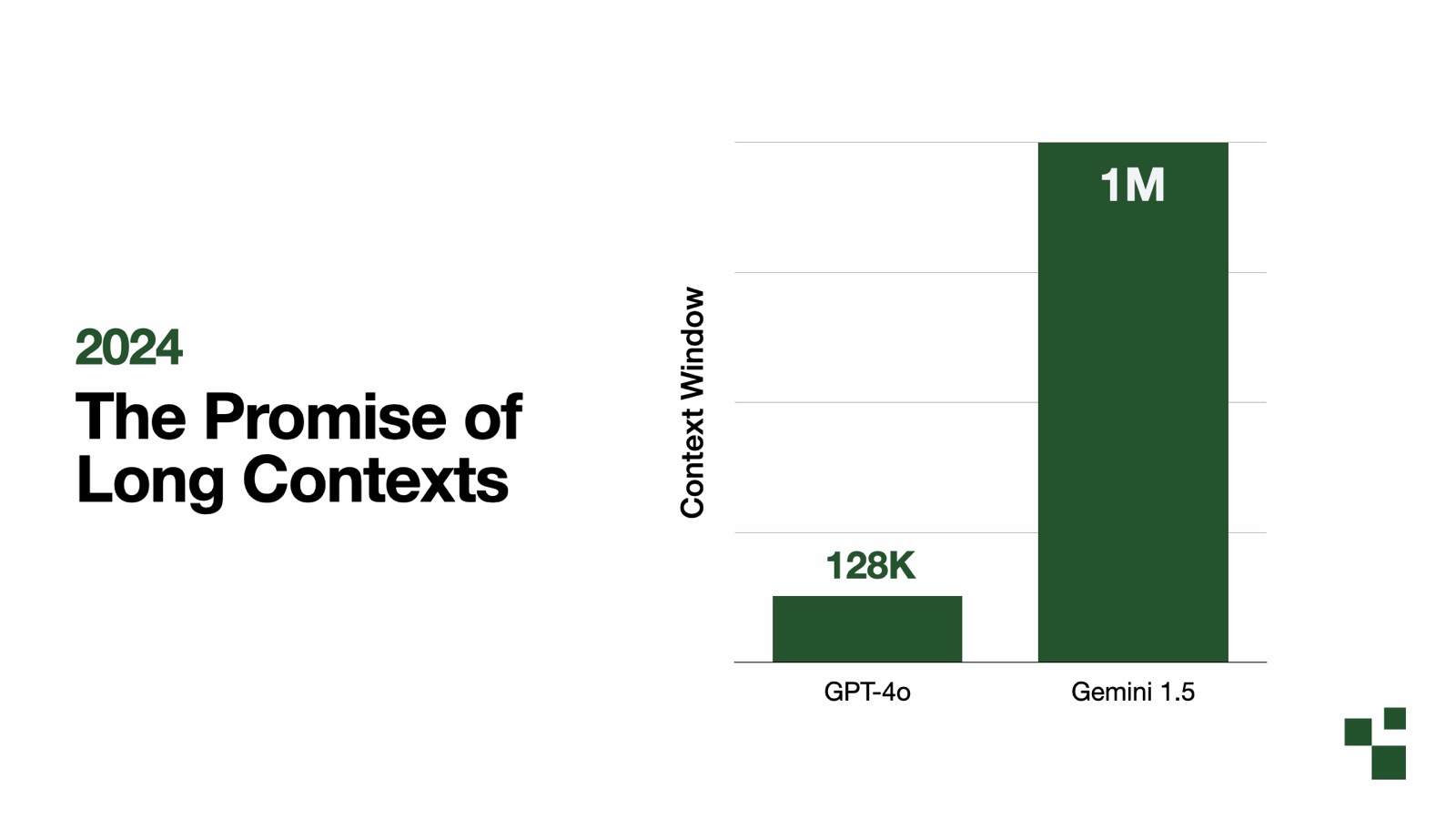
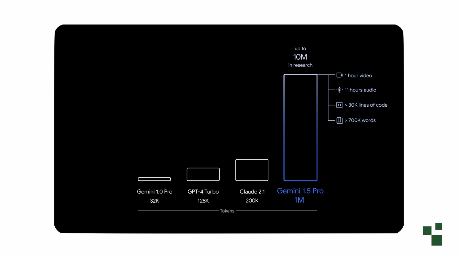
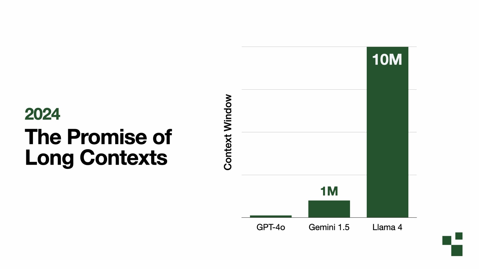



































![A breaking contract change: GET /brands no longer returns response[].name](https://github.com/winnin/farol/blob/main/docs/images/report-contracts.png)























![Side-by-side comparison. On the left, labeled “scalar”, eight separate ADD instructions stacked vertically, each adding one pair of numbers (1 + 10, 2 + 9, … 8 + 3) into a result of 11, with a clock next to every row and “8 instructions” at the bottom. On the right, labeled “SIMD”, a row a = [1 2 3 4 5 6 7 8] plus a row b = [10 9 8 7 6 5 4 3] produce a row of eight 11s at once, with a single clock and “1 instruction”.](https://internals-for-interns.com/images/go-simd-scalar-vs-simd.webp)

![A row of memory cells on top, labeled “memory: a []float32”, holding the values 1 2 3 4 5 6 7 8 9 10, with “addresses increase” pointing to the right. A brace under the first eight cells is labeled “32 contiguous bytes”, and a smaller grey brace under 9 and 10 says “left for next time”. A single arrow goes down from the first brace into a register Y0 drawn below, whose lanes, numbered 0 to 7, now contain 1 to 8, lane 0 holding a[0].](https://internals-for-interns.com/images/go-simd-load.webp)
![Two registers drawn one above the other: a = [1 2 3 4 5 6 7 8] and b = [10 9 8 7 6 5 4 3]. Between each pair of lanes is a small plus sign, and a straight vertical arrow runs from each lane pair down into a third register labeled a + b, holding [11 11 11 11 11 11 11 11]. Red vertical lines run through all three registers between every lane, walls that no value crosses.](https://internals-for-interns.com/images/go-simd-vertical-add.webp)
![A register at the bottom with eight lanes, labeled lane 0 to lane 7, each holding 11. A thick arrow goes up from it into an output slice labeled “out []float32”, eight contiguous memory cells indexed [0] to [7], each now holding 11.](https://internals-for-interns.com/images/go-simd-store.webp)

![A single small box labeled “a float32” holding the value 5, with eight red arrows fanning out from it into all eight lanes of a register, numbered 0 to 7, which becomes [5 5 5 5 5 5 5 5]. The register is labeled BroadcastFloat32x8(5).](https://internals-for-interns.com/images/go-simd-broadcast.webp)
![Two fused multiply-add steps stacked top to bottom, every register drawn as a row of eight lanes. Step 1, “acc = x1 · y1 + acc”: x1 = [1 2 3 4 5 6 7 8], y1 = [2 2 2 2 2 2 2 2] and acc = [0 0 0 0 0 0 0 0] flow down, lane by lane, into acc = [2 4 6 8 10 12 14 16], with the side note “1 × 2 + 0 = 2”. A red arrow labeled “reused” carries that result into the acc input of step 2, “acc = x2 · y2 + acc”: x2 = [8 7 6 5 4 3 2 1], y2 = [3 3 3 3 3 3 3 3] and acc = [2 4 6 8 10 12 14 16] flow down into acc = [26 25 24 23 22 21 20 19], with the side note “8 × 3 + 2 = 26”.](https://internals-for-interns.com/images/go-simd-fma.webp)
![Two registers a = [1 7 3 9 5 8 2 6] and a broadcast register [5 5 5 5 5 5 5 5] feed into a comparison labeled “a > 5”. The output is shown in two forms. On the AVX2 side, a full vector register whose lanes are either 0xFFFFFFFF (true, shaded) or 0x00000000 (false). On the AVX-512 side, a small k register holding just eight bits, 0 1 0 1 0 1 0 1 read from lane 0, one bit per lane.](https://internals-for-interns.com/images/go-simd-compare-mask.webp)
![Three registers stacked on top: x = [1 7 3 9 5 8 2 6], y = [0 0 0 0 0 0 0 0] and mask = [F T F T F T F T], with the T lanes in red. Below them, a result register labeled x.IfElse(mask, y) holding [0 7 0 9 0 8 0 6]. In the T lanes a solid red line comes down from x, past y and through the mask, into the result; in the F lanes a dashed black arrow comes down from y instead.](https://internals-for-interns.com/images/go-simd-blend.webp)
![On top, a source register x = [a b c d e f g h] with lanes numbered 0 to 7. In the middle, an index register [7 6 5 4 3 2 1 0]. On the bottom, a result register [h g f e d c b a]. Curved red arrows cross from the source lanes, through the index register, into the result lanes, reversing the order.](https://internals-for-interns.com/images/go-simd-permute.webp)
![Two four-lane registers, x = [1 2 3 4] and y = [5 6 7 8]. Red braces join neighboring lanes, 1 and 2, 3 and 4 in x, 5 and 6, 7 and 8 in y, and a red arrow with a plus sign goes from each pair into one result register [3 7 11 15]. The first two result lanes are marked “from x” and the last two “from y”.](https://internals-for-interns.com/images/go-simd-concat-add-pairs.webp)
![A memory row with the last two elements of a slice, 9 and 10, followed by cells marked with a question mark labeled “not ours: past the end of the slice”. A mask [T T F F F F F F] sits under it. Arrows show 9 and 10 going into lanes 0 and 1 of a register, while lanes 2 to 7 are filled with zeros. Labeled “partial load: 2 loaded, 6 zeroed”.](https://internals-for-interns.com/images/go-simd-partial-load.webp)

![A box “your code: func dot(a, b []float32) float32, uses simd.Float32s”. A thick arrow labeled “midway rewrite (compiler, after type checking)” leads down to a box “dot (dispatcher, same name)”. A small box “at startup: CPU features + GODEBUG=simd” points into the dispatcher. From the dispatcher, arrows go to four boxes in a two-by-two grid: dot@128 → Float32x4, dot@256 → Float32x8, dot@512 → Float32x16 and dot@emulated → pure Go. The arrow to dot@256 is thick and red, labeled “chosen on an AVX2 machine”.](https://internals-for-interns.com/images/go-simd-midway.webp)
![Step 1, “full chunk (a[0:8], b[0:8])”: x = [1 2 3 4 5 6 7 8] and y = [10 9 8 7 6 5 4 3] go through MulAdd into acc = [10 18 24 28 30 30 28 24].](https://internals-for-interns.com/images/go-simd-dot-step1.webp)
![Step 2, “tail (a[8:], b[8:])”: x = [9 10 0 0 0 0 0 0] and y = [2 1 0 0 0 0 0 0], with the six zero lanes shaded and labeled “six zero lanes (masked off)”. MulAdd updates acc to [28 28 24 28 30 30 28 24], with +18 and +10 marked over lanes 0 and 1.](https://internals-for-interns.com/images/go-simd-dot-step2.webp)
![Step 3, “fold”: acc = [28 28 24 28 30 30 28 24] is split into [28 28 24 28] and [30 30 28 24], which are added element-wise into [58 58 52 52]. ConcatAddPairs turns that into [116 104 116 104], and a second ConcatAddPairs into [220 220 220 220].](https://internals-for-interns.com/images/go-simd-dot-step3.webp)
![Step 4, “out”: the register [220 220 220 220] with lane 0 marked, and an arrow labeled “GetElem(0) — same as the scalar loop” pulling out a single 220, in red.](https://internals-for-interns.com/images/go-simd-dot-step4.webp)